Vectorized Automatic Differentiation

In the last post, we discussed techniques for computing derivatives (or gradients) of arbitrary computational functions, with automatic differentiation (AD) being the most generic approach; i.e., it works for any function, even those containing control flow statements like for-loops and if-conditions.

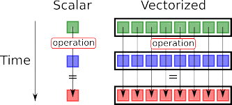
This post will discuss how we can vectorize that approach. Specifically, we will discuss vectorizing forward mode AD (although reverse mode AD can be vectorized in a similar way).

The examples shared in this post are from my implementation of vectorized forward mode AD in the Clad project, a source transformation based AD tool, as part of the Google Summer of Code program.

Recap of forward mode AD

Let’s briefly recap the basics of forward mode AD with an example, this will also help in building an intuition for the vectorized version.
Let’s consider a simple example:

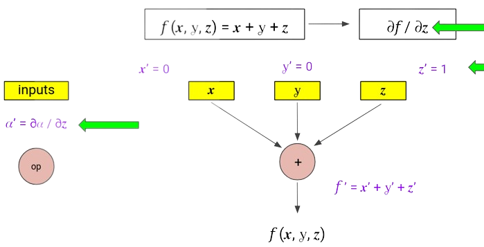
$$ \begin{align} f : \mathbb{R^3} &\rightarrow \mathbb{R} \newline f(x, y, z) &= x+y+z \newline \text{ compute } & \frac{\partial{f}}{\partial{x}} \end{align} $$

Steps for computing the derivating using forward mode AD,

• Form the computation graph, with nodes being inputs and the operators.

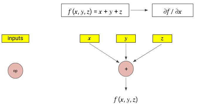
• Computing the function is equivalent to going through this graph in forward direction.
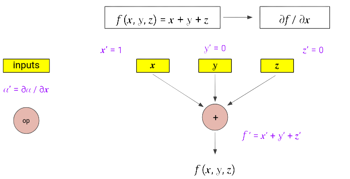
• Derivatives can also be computed in the similar fashion, difference being that each node computes $\frac{\partial{\text{ (node output) }}}{\partial{x}}$, thus propagating to $\frac{\partial{f}}{\partial{x}}$ in the end.
  • This means that each input node is initialized with a 0 or 1 value. (1 for input node $x$ as $\frac{\partial{x}}{\partial{x}} = 1$, whereas other input nodes are assigned 0 as the initial value).
  • At each operator node, we apply basic rules of differentiation (for example, using the sum rule at $+$ node and the product rule at $*$ node).

Computing $\frac{\partial{f}}{\partial{x}}$

Working Example

Let’s try to generate the derivative function for this example with clad:

double f(double x, double y, double z) {
  return x + y + z;
}

int main() {
  // Call clad to generate the derivative of f wrt x.
  auto f_dx_dz = clad::differentiate(f, "x");

  // Execute the generated derivative function.  
  double dx = f_dx.execute(/*x=*/ 3, /*y=*/4, /*z=*/ 5);
}

Function generated by clad for differentiating $f$ w.r.t $x$.

double f_darg0(double x, double y, double z) {
  double _d_x = 1;
  double _d_y = 0;
  double _d_z = 0;
  return _d_x + _d_y + _d_z;
}

Vectorized forward mode AD

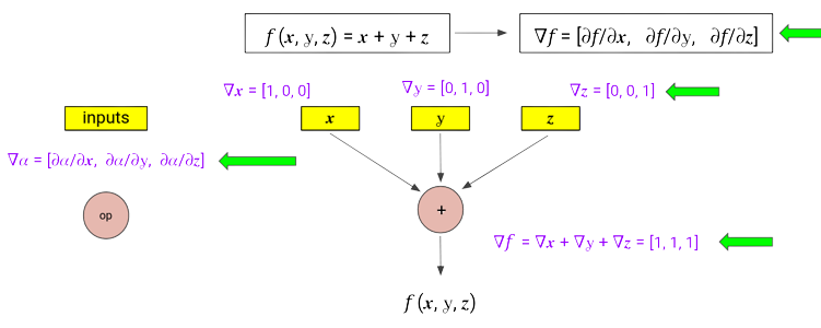
Now that we have seen how to compute $\frac{\partial{f}}{\partial{x}}$, how about computing $\frac{\partial{f}}{\partial{y}}$, and similarly $\frac{\partial{f}}{\partial{z}}$ ?

Computing $\frac{\partial{f}}{\partial{y}}$

---

Computing $\frac{\partial{f}}{\partial{z}}$

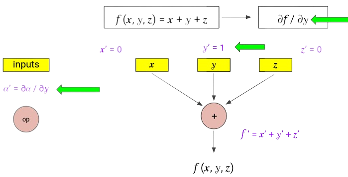
Although, the strategy is pretty similar, it requires 3 passes for computing partial derivatives w.r.t. the 3 scalar inputs of the function. Can we combine these?

• At each node, we maintain a vector, storing the complete gradient of that node’s output w.r.t. all the input parameters , $\nabla{n} = \left[ \frac{\partial{n}}{\partial{x}}, \frac{\partial{n}}{\partial{y}}, \frac{\partial{n}}{\partial{z}} \right]$ (where $n = \text{node output}$).
• All operations are now vector operations, for example, applying the sum rule will result in the addition of vectors.
• Initialization for input nodes is done using one-hot vectors.

Computing $\nabla{f}$

Defining the proposed solution

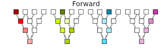
For computing the gradient of a function with $n$-dimensional input ($\in \mathbb{R^n}$) - forward mode requires n forward passes.

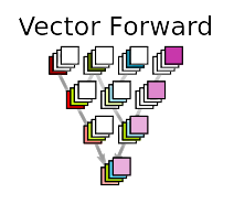
We can do this in a single forward pass, if instead of accumulating a single scalar value of the derivative with respect to a particular node, we maintain a gradient vector at each node.

$\rightarrow$

Reference: jnamaral.github.io

Working example

Same example function, but now computing $\frac{\partial{f}}{\partial{x}}$ and $\frac{\partial{f}}{\partial{z}}$ together.

double f(double x, double y, double z) {
  return x + y + z;
}

int main() {
  // Call clad to generate the derivative of f wrt x and z.
  auto f_dx_dz = clad::differentiate <clad::opts::vector_mode> (f, "x,z");

  // Execute the generated derivative function.  
  double dx = 0, dy = 0, dz = 0;
  f_dx.execute(/*x=*/ 3, /*y=*/4, /*z=*/ 5, &dx, &dz);
}

Function generated by clad for differentiating $f$ w.r.t. $x$ and $z$ using vector mode.

void f_dvec_0_2(double x, double y, double z, double *_d_x, double *_dz) {
  clad::array<double> d_vec_x = {1, 0};
  clad::array<double> d_vec_y = {0, 0}
  clad::array<double> d_vec_z = {0, 1};
  {
    clad::array<double> d_vec_ret = d_vec_x + d_vec_y + d_vec_z;
    *_d_x = d_vec_ret[0];
    *_d_z = d_vec_ret[1];
    return;
  }
}

Note that, now in a single forward pass, we can compute derivate w.r.t. multiple parameters together.
The main change in the interface is using the option clad::opts::vector_mode.

Benefits

Now that each node requires computing a vector, this requires more memory (and more time goes into these memory allocation calls), which must be offset by some improvement in the computing efficiency.

• This can prevent the re-computation of some expensive functions, which would have executed in a non-vectorized version due to multiple forward passes.
• This approach can take advantage of the hardware’s vectorization and parallelization capabilities (using SIMD techniques).

Progress in Clad

The complete progress report of this project along with the missing features and future goals can be seen here, and a basic documentation of using this vectorized mode is available here.

The following is a more complex example of differentiation functions consisting of array parameters using the vectorized forward mode AD implementation in Clad.

// A function fo weighted sum of array elements.
double weighted_sum(double* arr, double* weights, int n) {
  double res = 0;
  for (int i = 0; i < n; ++i) {
    res += weights[i] * arr[i];
  }
  return res;
}

Using Clad's vector mode for differentiating w.r.t. `arr` and `weights` parameters.

void weighted_sum_dvec_0_1(double *arr, double *weights, int n, clad::array_ref<double> _d_arr, clad::array_ref<double> _d_weights) {
  // Calculating total number of independent variables.
  unsigned long indepVarCount = _d_arr.size() + _d_weights.size();

  // Initializing each row with a one-hot vector is equivalent to initializing an
  // identity matrix (possible shifted and rectangular) for complete array.
  clad::matrix<double> _d_vector_arr     = clad::identity_matrix(_d_arr.size(), indepVarCount, 0UL);
  clad::matrix<double> _d_vector_weights = clad::identity_matrix(_d_weights.size(), indepVarCount, _d_arr.size());
  clad::array<int> _d_vector_n           = clad::zero_vector(indepVarCount);

  clad::array<double> _d_vector_res(clad::array<double>(indepVarCount, 0));
  double res = 0;

  {
    clad::array<int> _d_vector_i(clad::array<int>(indepVarCount, 0));
    for (int i = 0; i < n; ++i) {
      _d_vector_res += (_d_vector_weights[i]) * arr[i] + weights[i] * (_d_vector_arr[i]);
      res += weights[i] * arr[i];
    }
  }
  {
    clad::array<double> _d_vector_return(clad::array<double>(indepVarCount, _d_vector_res));
    _d_arr = _d_vector_return.slice(0UL, _d_arr.size());
    _d_weights = _d_vector_return.slice(_d_arr.size(), _d_weights.size());
    return;
  }
}