Automatic Differentiation

Given a continuos function $f(x)$, how do you compute it’s derivative $f’(x_0)$ for a particular input $x_0$ computationally?
Similarly, for a vector valued function $f(\vec{\boldsymbol{x}})$, how do we compute its gradient $\nabla_{\vec{\boldsymbol{x_0}}} f(\vec{\boldsymbol{x}})$? Where $\vec{\boldsymbol{x}}$ is an $n$ dimensional vector and

$$ \nabla f(\vec{\boldsymbol{x}}) = [ \frac{\partial f}{\partial x_0}, \frac{\partial f}{\partial x_1}, \dots \frac{\partial f}{\partial x_n}]^T $$

Computing these is beneficial in many applications - for example:

• Training of parameterized ML models (including Deep Neural Networks): this involves finding the optimal set of value of parameters $\boldsymbol{\hat{\theta}}$ which minimizes a particular loss function function $\mathcal{L}$ given a particular set of training examples $\boldsymbol{X}$ and corresponding labels $\boldsymbol{y}$, i.e:

$$ \begin{equation} \boldsymbol{\hat{\theta}} = \arg_{\theta} \min \mathcal{L} (\boldsymbol{X}, \boldsymbol{y}, \boldsymbol{\theta}) \end{equation} $$

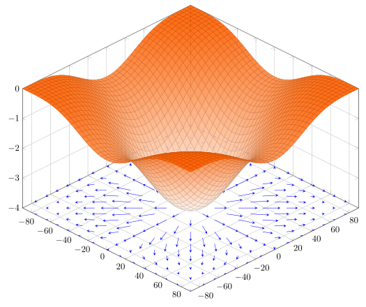
To solve the above optimization problem, we use some variant of gradient descent which exploits the property of gradient that it always points in the direction of maximum increase.
The optimization algorithm has the following iterative form:

$$ \begin{equation} \boldsymbol{\hat{\theta}}_{t+1} = \boldsymbol{\hat{\theta}}_{t} - \eta \nabla_{\hat{\theta}_t}\mathcal{L} (\boldsymbol{X}, \boldsymbol{y}, \theta) \end{equation} $$

The above equation essentially states that at each time step we move a little bit in the negative direction of the loss function’s gradient at the current estimate.

Numerical Differentiation

Well, we can start by the definition of the derivative:

$$ f’(x_0) = \lim_{h \rightarrow 0} \frac{f(x_0+h) - f(x_0)}{(x_0+h) - x} = \lim_{h \rightarrow 0} \frac{f(x_0+h) - f(x_0)}{h} $$

Now, using the above formulation we can compute the function $f$ at very small values of $h$, for example: $10^{-5}$.

This seems to be a good solution for cases where $f$ is sort of a black box function and we don’t have access to its inner details/compositions. But it has a major flaw:

for computing gradient of a $n$ dimensional vector valued function, it requires $2n$ computations of function $f$.

This can be particularly expensive for cases where $n$ is large, which is definitely the case for Deep Neural Networks based models.

Symbolic Differentiation

Treating $f$ as a black-box didn’t work out, this means we need to exploit how the function works internally - what are it’s individual smaller subfunctions for which $f$ is the composition.

For example: $$ \begin{align} \text{if } f(x) &= \log(x)\sin^2(x), \newline \Rightarrow f(x) &= f_1(x) \times f_2(f_3(x)) \newline \text{where } f_1(x) &= \log(x), f_2(x) = x^2, f_3(x) = \sin(x) \end{align} $$

Using the above structure, we can use the properties of derivatives like product rule and chain rule to compute the derivative of the complete function $f$ using the derivatives of $f_1, f_2, f_3$. This way we can get an exact expression of the derivative function $f’(x)$ using a rule based engine as follows:

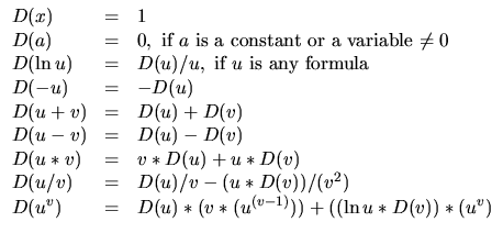
Rules for symbolic differentiation

This is what is used by tools like Wolfram Alpha.

• This seems like a perfect solution but the question is: do we want the complete expression of the derivative? For example: if $f$ is a product of $n$ such functions, then the derivative expression will contain $\approx 2^n$ terms, some of which may be redundant computations. One faces a similar problem when differentiating deep neural networks, which consists of composing many layers on top of each other.
• Although this method works for purely mathematical functions, but what about handling control flow? i.e how do we handle if conditions and for loops.

Automatic Differentiation

The aim is to get a procedure for computing the derivative of any general program. Hence, we come to Automatic Differentiation.

High level Idea

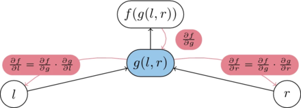
Automatic Differentiation (or AD or autodiff) breaks down the computation into a computation graph of primitive operations (like $+, -, \times, \div$) and some primitive functions (like $\sin, \cos, \exp$) and uses chain rule and other basic rules of differentation to compute the derivatives in a procedural manner.

Example Computation Graph

An example computation graph taken from Pytorch's blog

Forward Mode AD

In forward mode AD, the aim is to calculate the derivative of the ouput(s) with respect to any one input variable. This is done by calculating the derivative w.r.t that input at each node, starting from the input nodes and traversing in the toplogical order all the way upto all output nodes.

This way we are essentially computing $\frac{\partial n}{\partial x_i}$ for every node $n$, where $x_i$ is the input node related to which we want the derivative results.

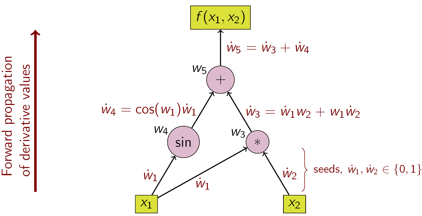
Forward mode AD example

Using forward mode AD for computing gradient of a function $f: \mathbb{R}^n \rightarrow \mathbb{R}^m$ will require $n$ traversals of the computation graph, i.e once for each input variable (although, we can vectorize this whole method which will be discussed in a future post).

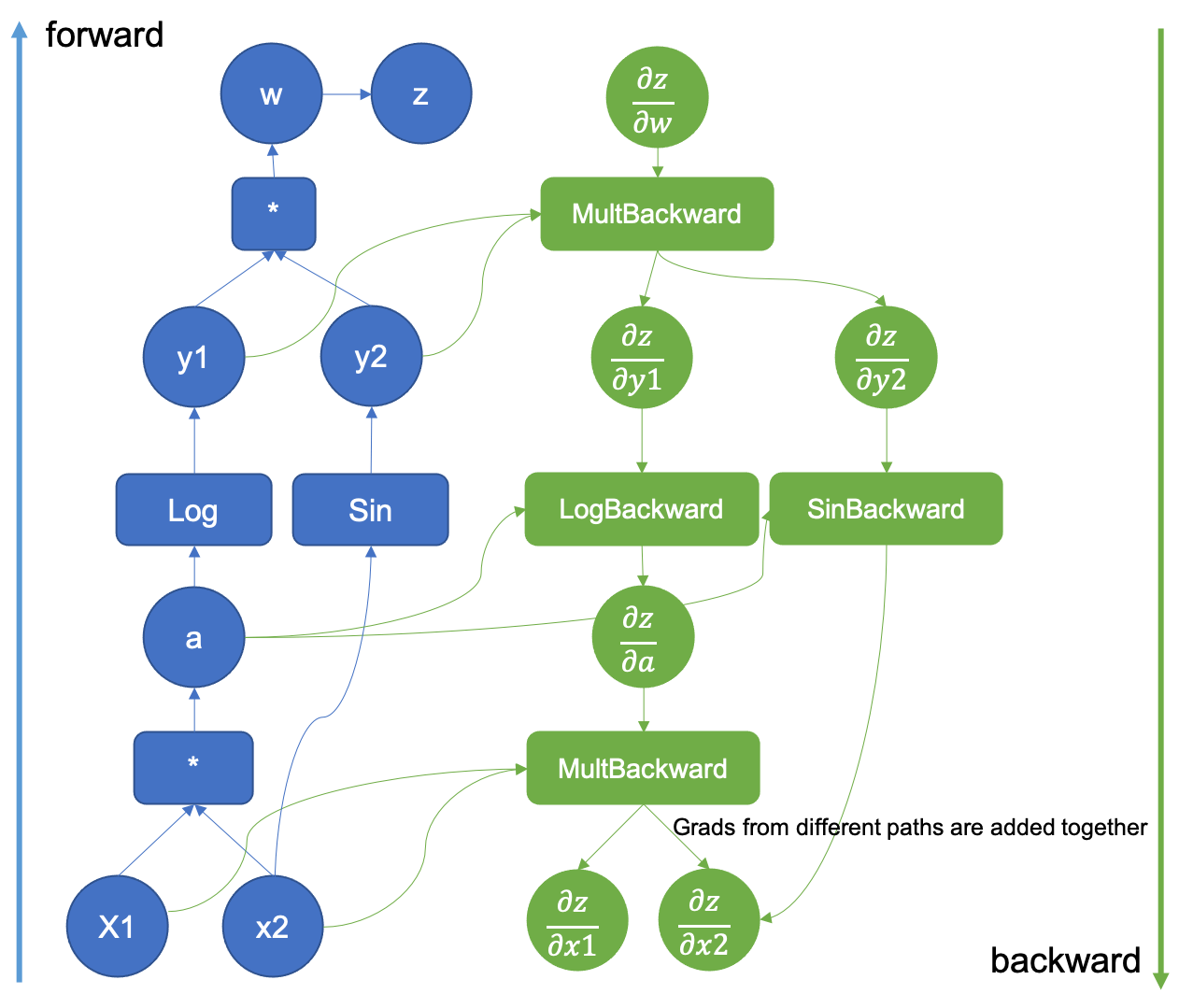
Reverse Mode AD

As the name suggests, this method is completely opposite of the fwd mode, the aim is to calculate the derivative of one ouput value with respect to all input variables. This is done by accumulating all the derivatives while going in reverse - from output nodes to input nodes.

Reverse accumulation of derivatives

In this method, we are essentially computing $\frac{\partial out_i}{\partial n}$ for every node $n$, where $output_i$ is the output node related to which we want the derivative results. This is done starting from the putput nodes and traversing in the reverse toplogical order all the way upto input nodes.

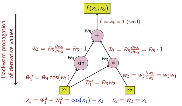
Reverse mode AD example

Using reverse mode AD for computing gradient of a function $f: \mathbb{R}^n \rightarrow \mathbb{R}^m$ will require $ms$ reverse traversals of the computation graph, i.e once for each output variable.

Reverse mode AD is particular helpful in cases where $m$ is very less, for example in deep neural networks the final ouput is a single scalar value of the loss function (hence $m$ = 1), that’s why deep learning libraries mainly use this mode for computing gradients w.r.t to all the parameters of the model.

Implementation strategies

There are mainly two ways of implementing AD, one works at runtime by overloading the operators used in the source function, this is the implementation approach used inside python libraries like autograd and deep learning frameworks like pytorch.
The other strategy is to use the AST of the source program for understanding the corresponding computational graph and build the AST for the derivative function, which is passed to the further stages of compilation to generate the code for the newly constructed AST.

Overloaded Operators

In this approach, all operations are performed on a custom defined class. This class makes sure to overload all the commonly used operators and functions for two main reasons:

• When computing the expressions, it makes sure to create a new object for every results which also keeps track of the inputs and operation used to produce this node. Hence, maintaining the computational graph. This looks very similar to the basic python snippet below:

  class Value:
      def __init__(self, data, parents=(), _op=''):
          self.data = data
          # internal variables used for graph construction
          self._prev = set(parents)
          self.function = _op # the operation that produced this node
  
      def __add__(self, other):
          out = Value(self.data + other.data, (self, other), 'add')
          return out
  

  Using this, when adding two Value objects, a new Value object is created which also keeps track of it’s input nodes.

• This also allows defining how gradients should be propagated for each particular operation/function (for both forward or reverse mode AD).

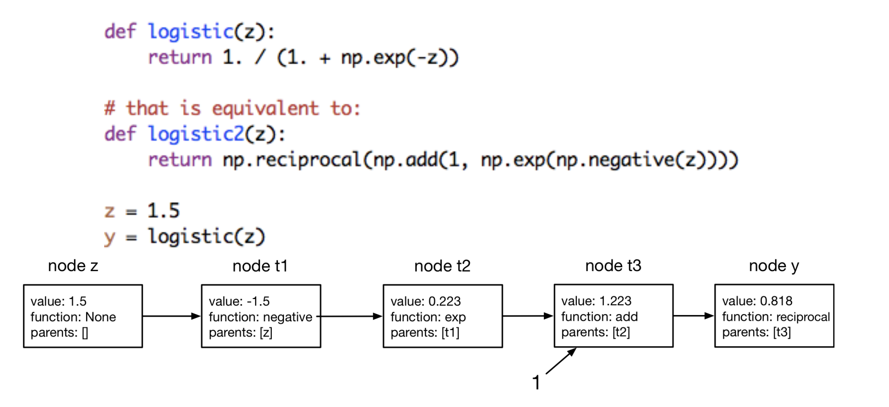
An example of how this might look like by overloading numpy operations (as done by autograd library).

Because the computation graph is formed dynamically at runtime, there is no need for the implementation to understand the control flow of the source program.

Source Code Transformation

In this approach, the source code of the program to be differentiated is traversed at compile time and a new function is automatically generated for the corresponding derivative code. Benefit of having this approach is that the generated code can take benfit of compiler based optimizations.

One example project for this on which I am contributing is clad. It is a clang plugin which constructs the computational graph by analysing the AST of the program and allows doing both forward or reverse mode AD for computing quantities like gradient and jacobian. For complete details on its working, you can refer to the documentation on the project page.

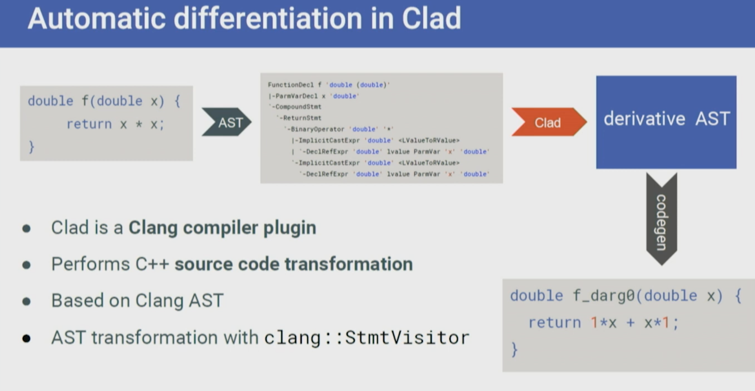
Overview of clad